Dijkstra’s Algorithm Tutorial with The Simpsons

Ever wondered how Google maps works out which route you should take to avoid the roadworks? Or how LinkedIn has an eerie habit of identifying the person you bumped into in the office earlier as a person you may know? Or how on earth Amazon thinks it can make deliveries possible via drones?

Today we’re going into the algorithms of just how I managed to plan Bart’s ideal trick or treating route around Springfield. 

How data science finds the optimal route…

One of my favourite data science topics is how resourceful we are. We combine tools from mathematics, statistics, computer science and sometimes even economics with domain specific knowledge and a tun of communication skills to translate problems to data to models to explanations. And today we’re going to dive into one of these topics in a little more detail to explain how it works. 

Back in October, I created the perfect Trick or Treating route for Bart Simpson using a combination of Dijkstra’s algorithm for pathfinding and orienteering algorithms for avoiding Sideshow Bob. So today I wanted to do a bit of a deep dive into each of these algorithms, explaining how they work and where you might end up using them when it comes to real life. 

So to kick it off, let’s start with a word I struggle to spell as much as I struggle to say it. Let’s talk about the algorithm that can get around the London tube map even more efficiently than me. Let’s talk about Dijkstra’s algorithm. 

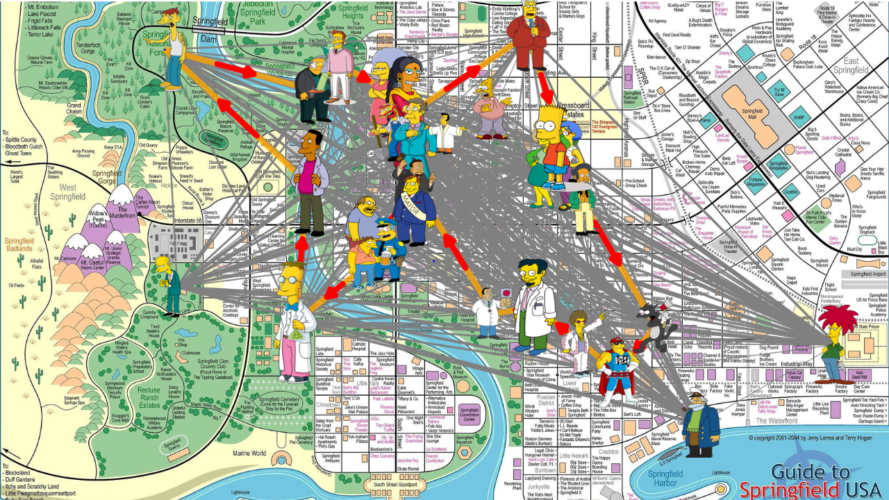
Graph showing how to find Barts optimal route

My First Encounter with Dijkstra’s Algorithm

So my first encounter with Dijkstra’s algorithm was actually in a further maths class at school. I remember being incredibly confused as to why we were finding the shortest route through an arbitrary graph by hand when it didn’t seem like particularly advanced maths so I wanted to start by giving you the context I wish I’d had then. 

So Dijkstra’s algorithm by definition is a methodology for finding the shortest path between any two nodes in a weighted graph which when phrased like that, is incredibly abstract. So let’s start out by defining what some of those terms are by using, for the fourth video I’ve got out of this one topic, my map of Springfield. 

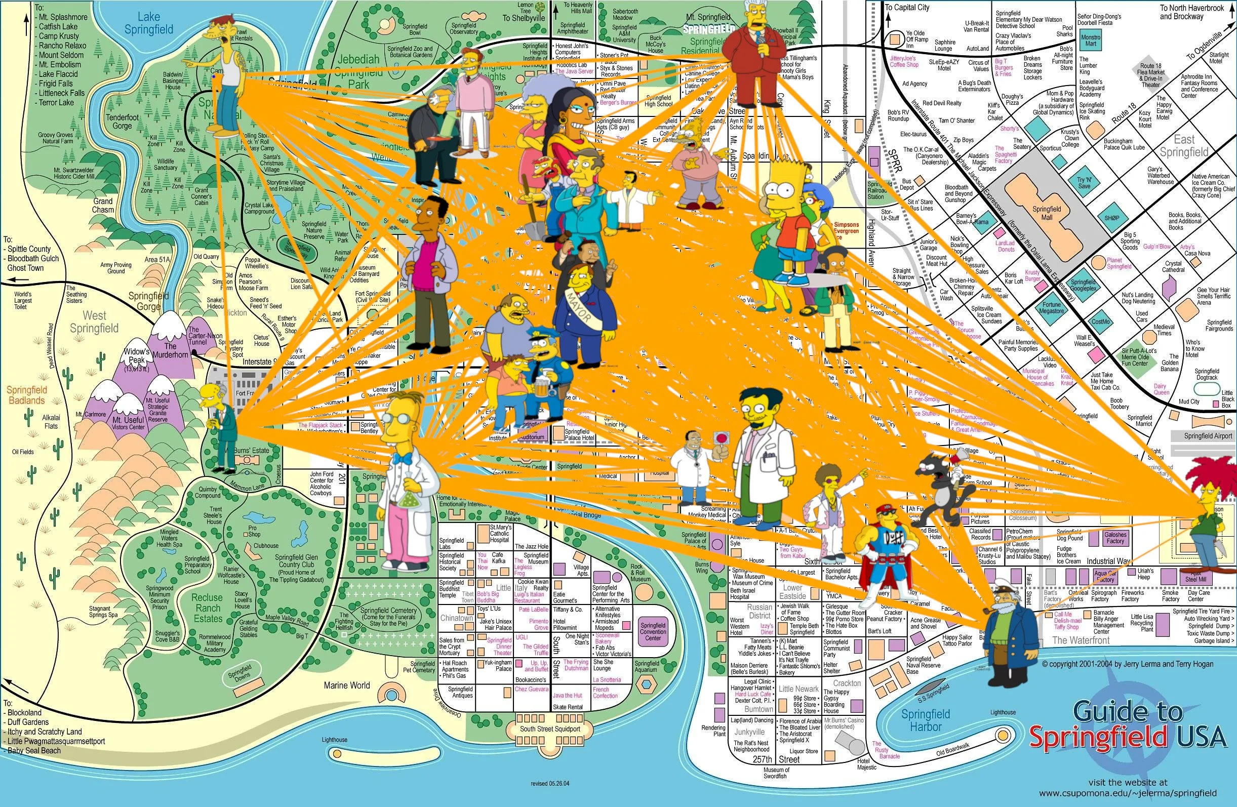
Below is the map of Springfield. In a previous video, I explained the process of identifying the characters I wanted to highlight and converting that data into a computer readable format. If you’d like more detail, you can watch that video but for now, here’s how everything is set up

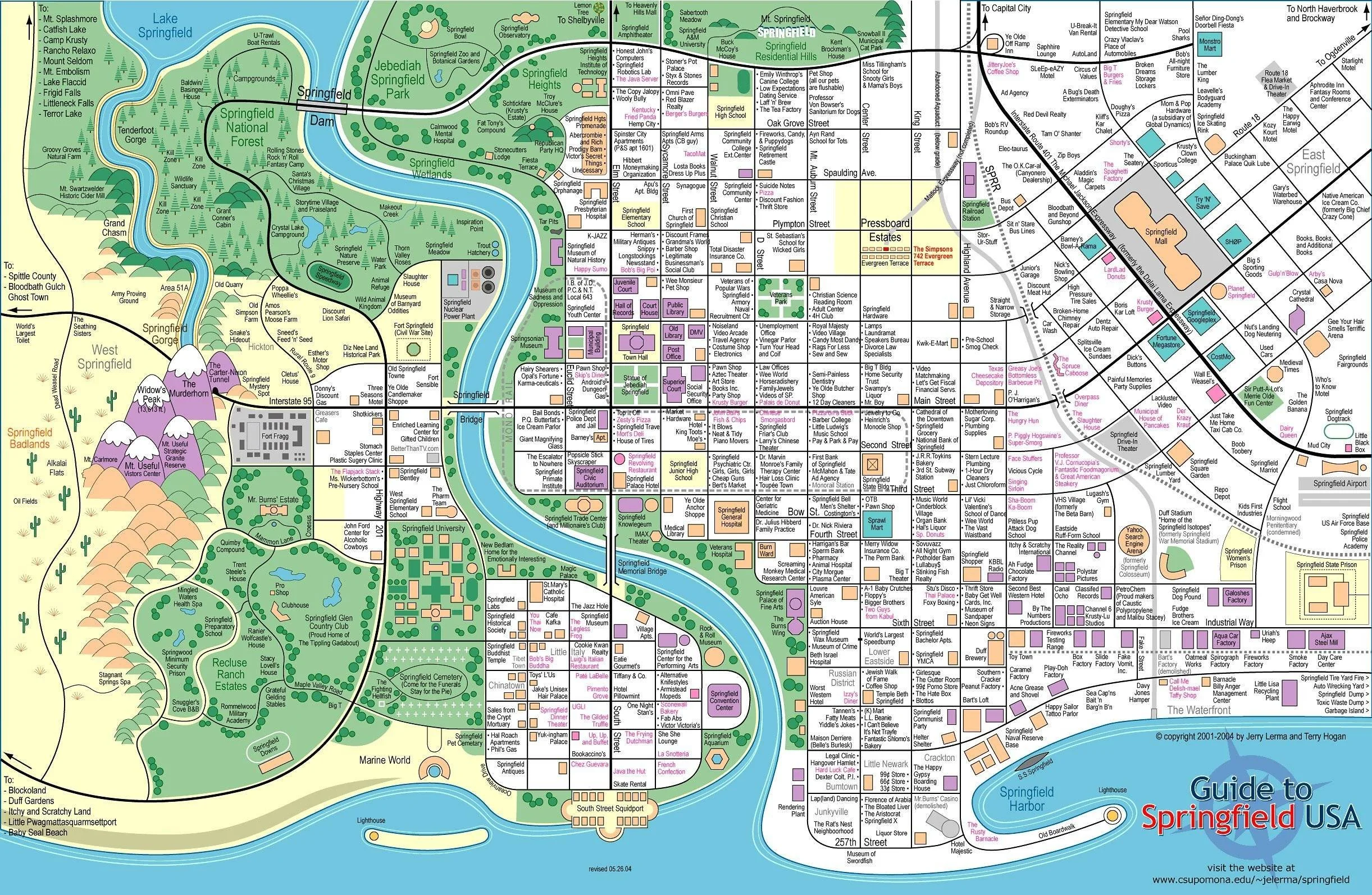
Map of Springfield

From Map to Graph: Nodes and Edges

I’ve marked each character on my map and they’re given by nodes. They’re not the only nodes but they’re the points that I care about and they make up the main points of my graph. 

In order for a graph to become a graph however, I also need edges and those are the roads of Springfield. If all these roads were straight lines that connected one character to another, my graph would be complete but reality doesn’t work like that. As in any real city, in Springfield we have corners and intersections and to capture that complexity I turned each intersection into a node and then connected them by the paths between them. 

I also added zero-weight connectors to make up for my lazy character plotting earlier. You’ll be able to spot them because they look a lot less… artistic shall we say?

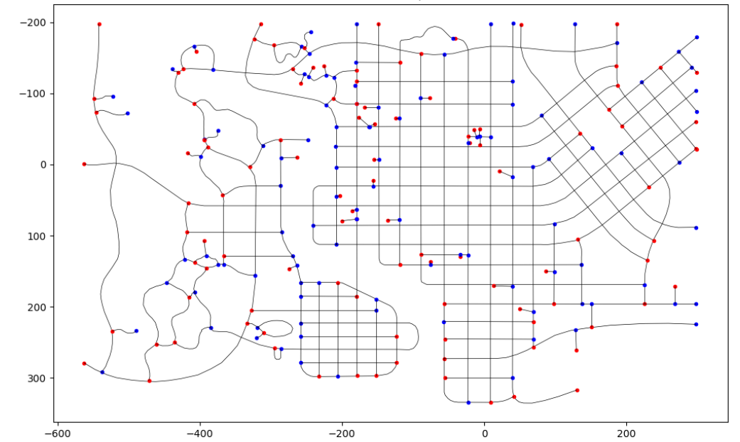
Graph of Springfield showing nodes and zero-weight connectors

By building up the whole graph this way I have something that looks like this: 

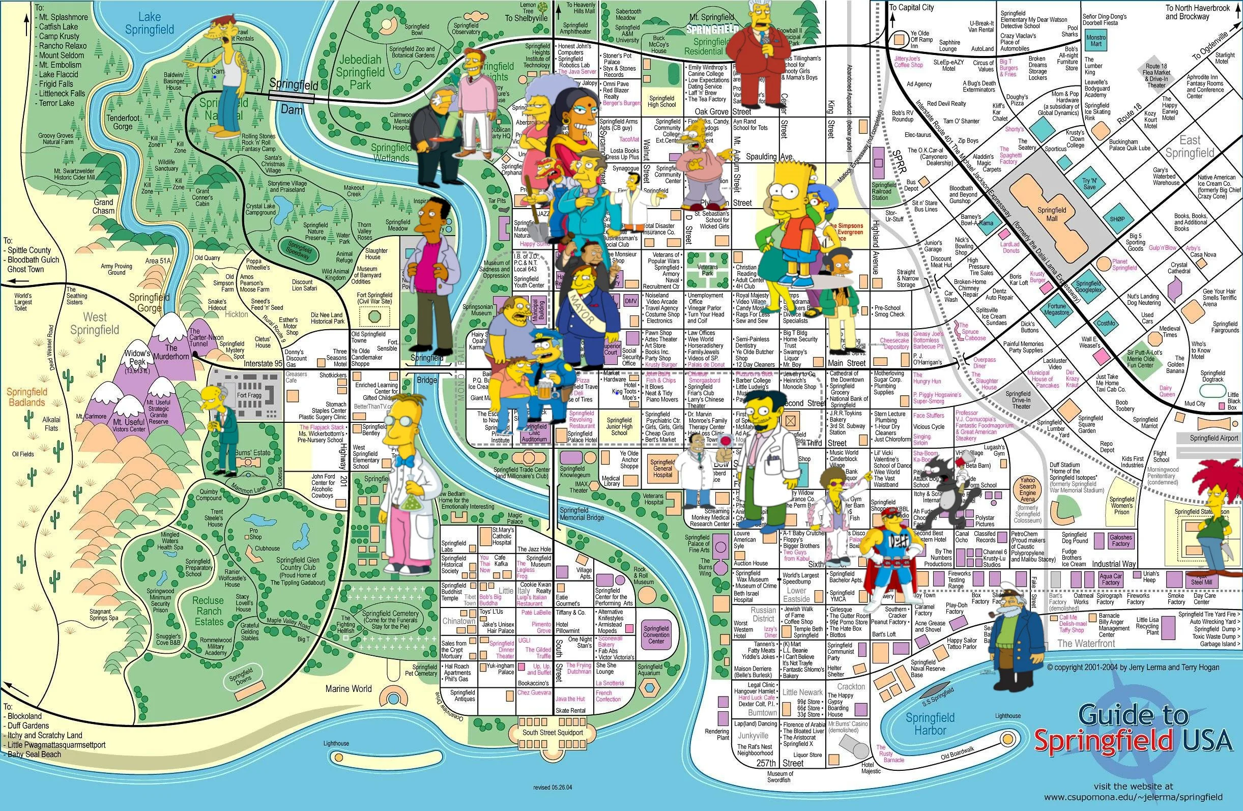
Map of Springfield showing characters plotted on the map of their locations

And you can see from this graph that there are thousands of ways we could get between Bart and Abe Simpson with routes that make sense to ones that zig zag through the neighbourhood but ultimately are fine to ones that create massive unnecessary detours, maybe even swinging by the prison to goad Sideshow Bob. 

And that’s a problem, because much like your commute to work, you probably want to find the shortest way to get there. That’s where Dijkstra’s comes in. 

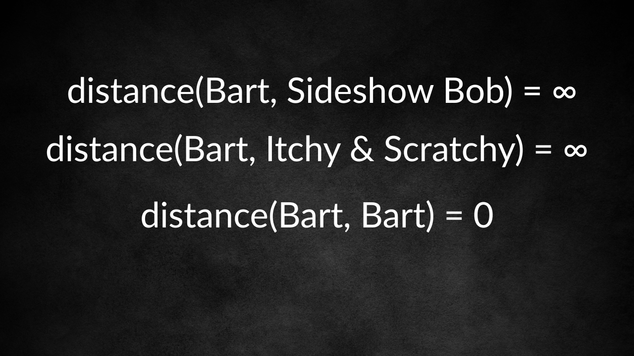
So let me break down how this algorithm works. We start by creating a set of all nodes we haven’t been to yet, called the unvisted nodes, and we dub the distance to those nodes to be infinite because we haven’t found a shortest path to the node yet. Our start node is set to have distance of zero because we’re just starting there. 

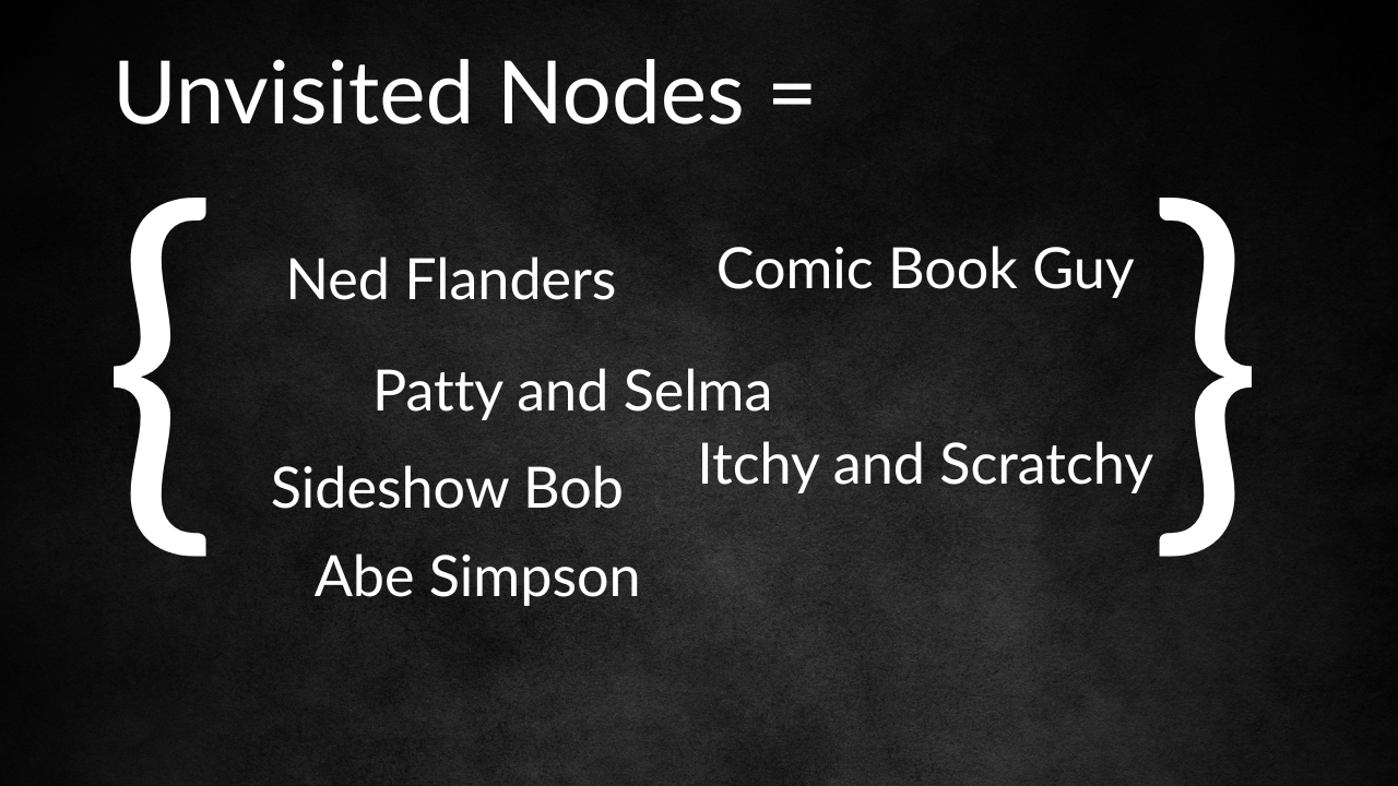
Unvisited Nodes list

Breakdown of Dijkstra Algorithm

We then look at the unvisited set and choose where to go next. Our choice is the node with the smallest unvisited distance. So in our case because we have connector paths of length zero, we’re going to go immediately from Bart to the end of the connector path. If we’re at our target end node we stop there, but we aren’t, so we keep going.

Now for the current node, the one at the end of the connector, let’s call it node A, we consider all of it’s unvisited neighbours and see if they already have a path stored. Let’s say we’re currently looking at node B. 

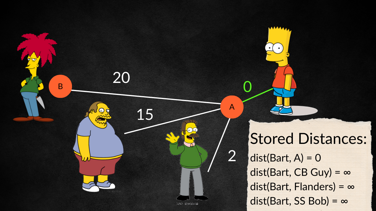
Diagram showing the connecting of nodes and their stored distances

We check if we already have a path from Bart to B already calculated. If not, we store this distance as our shortest path from Bart to B. But if we do, we need to make a decision. If this new path, Bart A B is a shorter path than the currently stored path which might go Bart F K L B, we throw that path out and store this new path Bart A B instead. If it’s worse, then we keep the older path. 

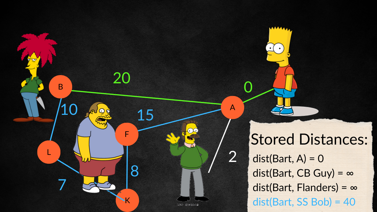
Diagram showing the connecting of nodes and their stored distances

After we’ve done this for every node that connects to A, we can consider A a fully visited neighbour and remove it from our unvisited set - we don’t want to visit a node we’ve already been to already. 

We continue these steps until we have completed node Abe Simpson and removed it from the unvisited nodes set. At that point, whatever is in our slot as the shortest distance from Bart to Abe Simpson is noted down as our shortest path.

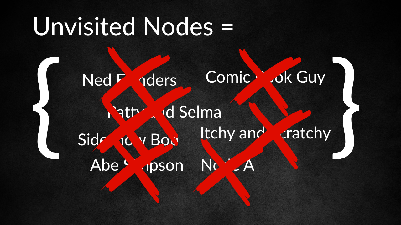
Unvisited nodes set - completed

So this is great, if I know the shortest distance from Bart to Abe Simpson, then I don’t actually need all other paths between the two of them, in fact, I could just chuck out those paths and replace them with a straight line connecting the two, as long as I labelled the distance to be the one given by Dijkstra’s. If I do this between all Simpsons pairs, I go from a crazy graph with loads of nodes to one that only contains my 32 Simpsons characters of interest. 

But that didn’t solve my trick or treating problem, did it? Because sure, I know the fastest way Bart can get to all characters, but if he has to backtrack home every time he’s wasting valuable candy collecting time. And I’m pretty sure he doesn’t actually want to go visit Sideshow Bob. 

Map of Springfield showing the characters of interest and their connecting paths

Faster, Better, Smarter: Algorithms That Save Time

It was here that I introduced the concepts of penalties and rewards, literal tricks and treats we can use in an algorithm to create a trick or treating route for Bart. So much like how city mapper gives you an alternate route when the northern line is down, we’re going to use orienteering algorithms to save Bart travel time and maximise his candy collection. 

And if YOU want to save the time you waste waiting for your code to run, our platform was designed by data scientists for data scientists to decimate your wait time. Through better caching, multithreading and spotting those bugs you’re always annoyed at yourself for making BEFORE you’ve sent 2.3 million rows through the model. 

We’re launching a closed beta next month so click here to sign up.

Oh and before you go, there’s a massive penalty incurred if you don’t go over to our You tube channel and hitting like and subscribe so you better do that. There might even be a reward in it too. 

For more of this, come on the journey with us and keep being Evil