
Don't Let Text Data Blow Up Your Model. TF-IDF and Truncated SVD Tutorial
Not many people realise this but your favourite LLM can't actually be your therapist. Because a therapist understands what you mean. An LLM processes what you wrote. There's a difference.
You read "I feel lonely" and hear fear, grief, and a need for connection. A model reads tokens.
Words, to a model, are useless. Until you convert them. That conversion is what today's video is about. If you get that conversion wrong, you get a model that spouts nonsense or sees the word "and" as the ultimate predictor of customer churn. If you get it right, everything becomes possible.
So how do you actually do it?
How do you take a hundred film synopses and turn them into numbers that capture meaning?
Two tools. TF-IDF and Truncated SVD. Let's do some Evil Work.
The simplest way to represent text is a bag-of-words: count how many times each word appears in a document, put those counts in a vector.
Take the plot summary of Psycho (1960) as an example and it looks like this:
The problem is immediate. The word `the` scores highest. So does `and`, `to`. These words carry zero information about what this movie is about. They're just grammatical glue.
The standard fix is to remove stop words, a hand-crafted list of common words to ignore. that helps. But it doesn't solve a deeper problem: Frequency still doesn't mean importance.
Take the word “young,” for example. It might show up 120 times across a bunch of movie scripts, but that doesn’t mean the word is central to the story or changes anything about the plot.
Image showing the most frequently used words in Psycho by Alfred Hitchcock
word count, but doesn’t highlight the plot specific words
What we actually want is:
How much does a word show up here?
How rare is this word across all documents?
A word that's frequent in one document but rare everywhere else is a strong, specific signal. That's TF-IDF . Where TF is ”Term frequency", how often the word appears in this document, and IDF is "inverse document frequency" as a proportion of general documents.
Now let’s build this step by step.
First question: How much does a word show up here?
At first glance, you might just count how many times it appears. But that immediately creates a problem. Longer documents will always have higher counts, but that doesn’t mean the document is more about that word.
So instead, we scale the count by the total number of words in the document.
Term Frequency: TF(t, d) = f(t, d) / Σ_{t' ∈ d} f(t', d)
TF(t,d) = f(t,d), the frequency of term t in document d, divided by the sum of frequencies for all terms t.
sum for TF-IDF
Normalising turns counts into proportions. Now we’re comparing usage, not length.
So instead of asking: “How many times does this word appear?” We are asking “How much of this document is this word?”
In Psycho movie the 118-word synopsis has:
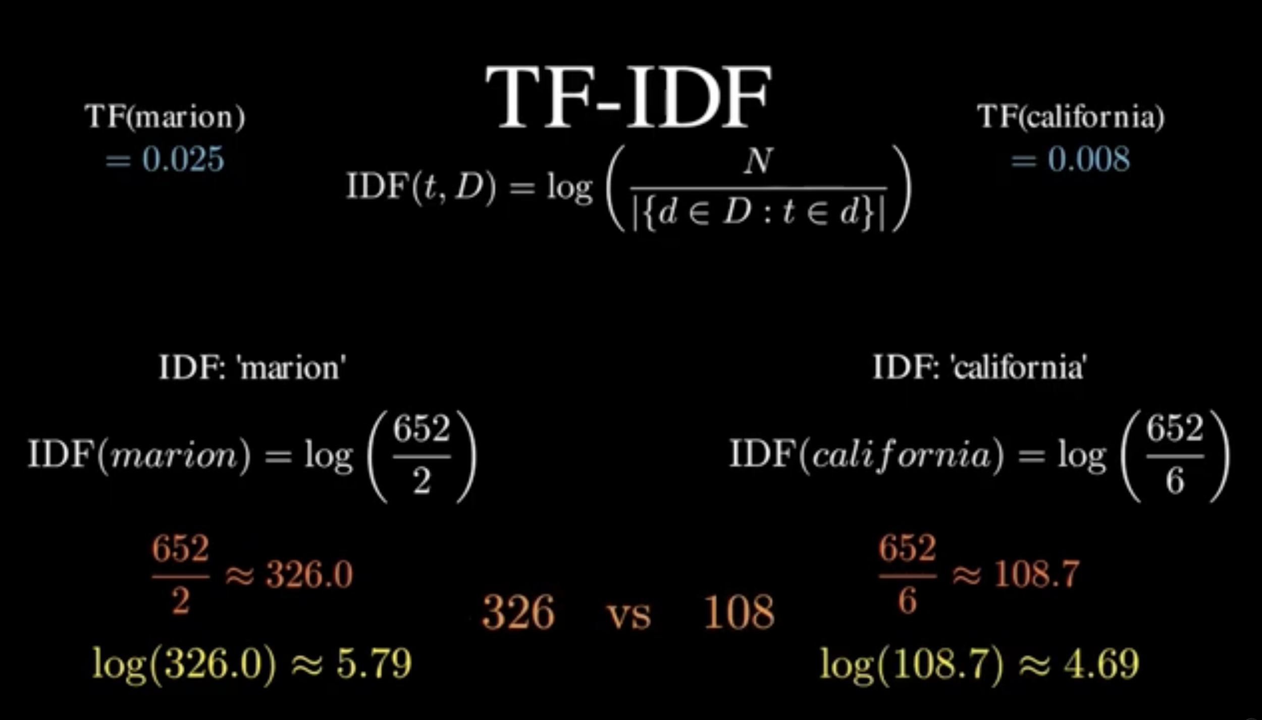
marion: 3 - 0.025
california : 1 - 0.008
So “marion” is more central within this document. But this is still local.
Now zoom out.
Second question: How rare is this word across all documents?
Inverse Document Frequency: IDF(t, D) = log( N / |{d ∈ D : t ∈ d}| ) Log of: N, the total documents, divided by the number of documents that contain this term.
This is measuring: Does this word show up everywhere, or is it specific? But here’s the problem. Before the log, this formula is like a completely broken volume knob.
Rare words are blasting at maximum volume. Slightly less rare words are way quieter.
Common words get turned down. Rare words get turned up. But nothing blows out your speakers. That's the IDF.
So now we can separate common words with low scores and rare words with high value. Now combine both ideas.
The TF-IDF is the TF multiplied by the IDF.
the score: TF-IDF(t, d, D) = TF(t, d) × IDF(t, D)
This creates a filter:
A word only scores high if:
it’s frequent here
and rare globally
Take “marion” vs “california”.
“California” appears in more movies overall so its IDF is lower.
“Marion” appears in fewer movies so its IDF is higher.
But that’s only half the story. If “Marion” shows up a lot in this synopsis, it will still get a decent score.
If “California” barely appears, its score drops. We’re close. But one last issue.
Now we have a number for every word, in every film. We assemble everything. Each document is a vector. Stack them together to make a matrix.
X ∈ ℝ^(N × m)
So what are we actually working with?
A matrix X where:
Five hundred and sixty two rows: one for each horror movie.
Three thousand, five hundred and forty five columns: one for each word.
Most of those columns are zero. Even a single synopsis already feels noisy and like a word cloud where every word is fighting for attention, with no clear signal.
Now imagine handing that to a model. Three thousand columns per movie, mostly empty, and it has to figure out what The Ring has in common with The Witch from that mess. It'll latch onto accidents. One film used "seven days." Another used "estate." Now those are load-bearing.
And here's the deeper problem: we don't actually care about individual words. We care about what kind of film this is. Gory. Psychological. Supernatural. Those are themes and themes live in clusters of related words, not individual cells of a matrix.
So instead of asking "which words appear," we want to ask: what direction is this movie pointing? We don't care how long a synopsis is. A two-sentence summary and a ten-sentence summary of the same film should land in the same place. We care about the direction of what the document is about.
This representation is too big. Too sparse. Too noisy. We need to compress it without losing meaning.
That's what SVD does. It takes the important parts and leaves out the noise. But that's not all. It also helps us find the shape hiding deeper inside the data.
Because words don’t appear randomly. "Knife" and "stab" tend to appear in the same films. "zombie" and "undead" do too. These words are correlated. These correlations mean the data doesn't spread evenly through all 3,000 dimensions. It clusters along a low-dimensional structure.
Instead of thinking in words, think in patterns of words. Single Value Decomposition finds those patterns and isolates the ones that are most important. The first direction captures the most variance in the data. The second captures most of what's left, and is constrained to be perpendicular to the first. And so on.
And what makes SVD so powerful is that it works with any real matrix X ∈ ℝ^(N × m):
X = U Σ Vᵀ
Think of it like this:
Each column of V is a weighted combination of words. That combination defines a “theme”. Each row of U tells you how strongly a document aligns with each theme.
Σ scales everything by importance.
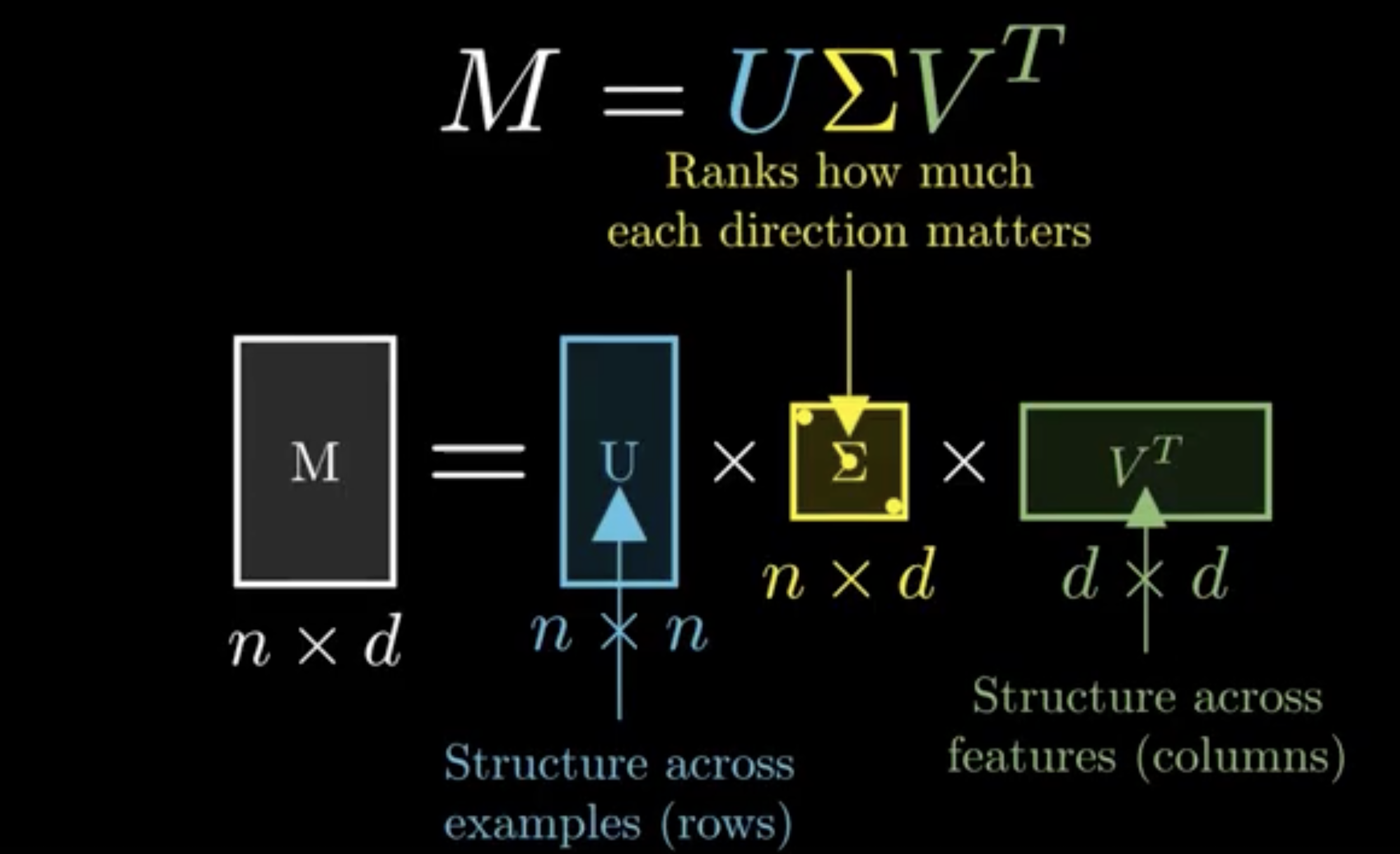
For instance, imagine the first direction (v₁) has 70% weight on “blood,” 20% on “gore,” and 10% on “slash.” This direction effectively represents the “slasher movie” theme. Movies that score highly on the corresponding coordinate (u₁) will cluster together, reflecting their shared underlying pattern of word usage.
Here’s the key insight:
Not all components matter equally. The singular values in Σ are not random. They’re ordered. Big ones at the top. Tiny ones at the bottom. That ordering is telling us something:
How much real structure lives in each direction.
The top components capture patterns that show up again and again across many films. The bottom ones? Mostly noise.
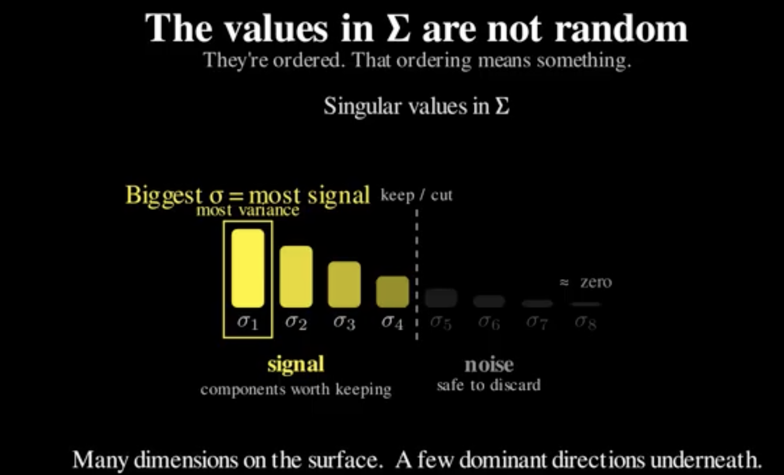
So instead of keeping everything, we keep only the top k components:
X̃ = U_k Σ_k V_kᵀ
Now three things happen at once:
Reduce dimensionality : 3,000 dimensions down to 20
Remove noise : by dropping the components with tiny singular values.
Keep the strongest structure : the themes that actually explain the data
It’s the best possible rank-k approximation of the matrix. Nothing else preserves more information in k dimensions. Now we take the result of that compression Z:
Z = U_k Σ_k
This is the embedding matrix. Each row is now a document. But look at what changed.
Before:
each dimension = a word
mostly zeros
hard to compare
Now:
each dimension = a theme
dense values
meaningful geometry
Each number now answers:
“How much does this document express this pattern?”
So instead of saying:
“This document has 3 occurrences of ‘marion’…”
We’re saying:
“This document strongly expresses the ‘serial killer investigation’ theme.” That’s a completely different level of abstraction. And this creates something powerful: A space.
In that space:
similar films land close together
different films land far apart
clusters emerge naturally
Distance now has meaning. Not just mathematically but semantically. That’s what an embedding is. It’s a representation where geometry = meaning. TF-IDF and Truncated SVD(under the name Latent Semantic Analysis) were powering real systems long before modern deep learning.
Search engines used it. Recommendation systems used it. Because the idea is simple:
The decomposition doesn’t care what the matrix means. It just finds structure. In our case, that structure came from horror movie synopses.
In the real world, it might be:
customer support tickets: cluster complaints into hidden issue types
legal documents: map contracts into theme space and flag anomalies
job postings: extract skill dimensions and match candidates by proximity
The pipeline is always the same:
raw text → TF-IDF → SVD → embeddings → model
The important part is understanding why each step exists.
Why do we normalise?
Why do we take logs?
Why do we truncate?
Because when something breaks when distributions shift, when recommendations look wrong, when performance drops the person who built a black box is stuck.
The person who understands the pipeline has somewhere to start.
Our closed beta launches this month. Sign up via the link below and keep being Evil