Feature Engineering: A beginner’s guide

After way too long looking you finally find a dataset you actually could use for your model. You download it, open the CSV and

Well... it's a mess. 

You know the information you need is in there somewhere but actually turning this into something you can use is intimidating at best and might kill your project before you even get started. 

Today I’m going to walk you through the exact first steps. 

How you take raw, messy columns and turn them into something a machine learning model can actually learn from. 

Because this is where most people get stuck. Not on the modelling part and its on the step before it: understanding the dataset well enough to turn it into useful inputs.

That skill is called feature engineering, and it’s massively underrated. You can throw the fanciest algorithm at a dataset but if the inputs are weak, the output will be weak too, just faster, and with more confidence.

And here’s the uncomfortable truth: most of the time, your model isn’t the problem. Your features are.

Stay with me, because I’m going to do a straight-up before-and-after. 

Baseline model first: meh. Then we do feature engineering (no new data, no fancy algorithm) and you’ll see the metrics move and the model’s behaviour change. It’s the difference between ‘it runs’ and ‘it works.

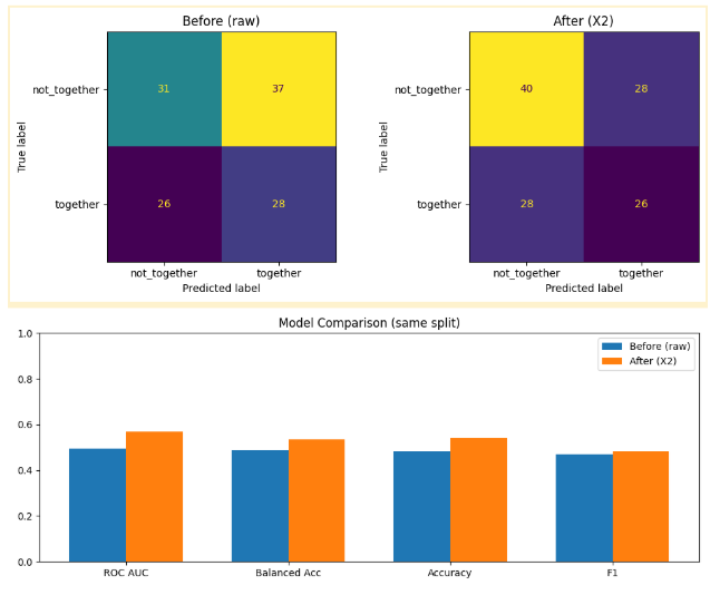
Graph’s showing the models before and after

So before we start creating anything new, we need to cover two quick basics:

• what feature engineering is,

• what data types we’re working with.

At its simplest, feature engineering is just this: turning raw columns into clear, structured signals a model can use.

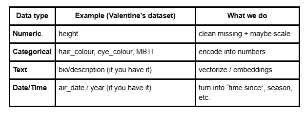
Table showing data types

And that’s the key idea: models can’t learn from raw labels and they learn from structured, numerical signals.

I'm going to show you exactly how to convert your raw labels into structured numerical signals, but first we're going to look at when it all goes wrong. I'm going to build a bad model. Intentionally this time! 

But first, quick context on the dataset: each row represents a TV couple.

 We’ve got both people in the relationship (things like height, hair and eye colour, personality type) and then the relationship outcome.

For this first baseline model, we’re going to use relationship status as the target we’re trying to predict.  

Then we build a simple pipeline to pre-process the data, choose Logistic Regression as our starter model, and split everything into train and test sets to evaluate how well it performs.
And here's the interesting part: once it’s trained, we can look inside the model and see what it thinks matters most and which features are pushing predictions toward “dating”, “married”, “broken up”, and so on.

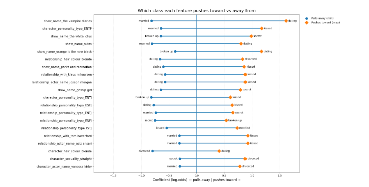
Graph showing the different features the classes push towards or away from

For example, imagine I tell you a couple is from The Vampire Diaries. The model instantly leans toward “dating.” Not because it learned anything real about relationships but because that show is written that way. 

It’s like predicting the ending of a movie because you recognize the studio and not because you understand the plot.

And then you see stuff that’s even more dangerous. Like hair colour. If the model is basically saying, “if they’re blonde, they’re more likely divorced,” that’s obviously not a real relationship rule. 

What’s actually happening is probably just a coincidence in the dataset and maybe one show has a divorced blonde character, and the model over-learns it.

Same with personality type. If the model sees one person is an ENTP and starts leaning toward “kissed” instead of “married,” that’s a red flag. 

Because relationships aren’t determined by one person’s label and they’re about the match between two people. 

So this isn’t “psychology”, it’s the model picking up character tropes and showing patterns in our data.

So what we’ve learned is: if you let the model, it’ll happily memorise shortcuts (show names, character tropes, random correlations) because that’s the easiest path to a prediction.

But it’s not really comparing the couple at all.

 To do that, we need to start feature engineering and building features that describe the relationship between two people, not just who they are individually.

And for that I’m going to get a little help.

• Relationship status

• Height difference 

• Personality type

• Same hair, same eye colour

Originally the dataset had multiple relationship outcomes: married, dating, kissed, secret, divorced, broken up. 

For the first version of this model, I mapped them into two groups:

• together: married, dating, kissed

• not_together: secret, divorced, broken up

And once the target was defined, the next problem was the inputs. Because the dataset was full of ‘person A’ and ‘person B’ columns and the model doesn’t naturally understand relationships. 

For example: we had two separate columns: person A’s height and person B’s height. But a model won’t automatically compare them. So I engineered a real pair feature:
height_diff_cm = |height_A − height_B|
Now it describes the couple, not the individuals.

Height was easy. Two numbers, compare them. But MBTI? That’s where it gets spicy.

Because if you just one-hot encode ‘ENTP’, ‘INFP’ and all that. The model treats it like a stereotype sticker. And I’m not even going to pretend I naturally understand what ‘ENTP’ means on sight.

So instead of asking the model to learn labels, I made it learn similarity.” “MBTI is just four letters that come from four yes/no dimensions:

 E/I, S/N, T/F, J/P.

So I cleaned the strings, made sure they’re valid 4-letter types, and then compared person A vs person B letter by letter. 

Each mismatch adds 1 point, so you get:

• mbti_diff_count = 0 to 4

0 means identical type, 4 means total opposites.
Now MBTI becomes ‘how similar are these two people?’.

Next I wanted a more human signal, so I borrowed an external MBTI compatibility table that says, for each type, which other types tend to be best, average, one-sided, or worst matches.

Instead of making the model learn every possible MBTI pair (all 16×16 combinations) I collapsed each couple into one clean label: compat_simple (best, average, one_sided, worst). 

Way less noise, way more signal.

Then I turned that into a number so the model can learn it:

• best = 1

• average = 2

• one_sided = 3

• worst = 4

Now the model can pick up a simple pattern: as compatibility gets worse, the chance of staying together should drop.

And after that, I added a few “cheap but effective” pair features and the kind that take seconds but often matter:

• eye_same: same eye colour? (1/0)

• hair_same: same hair colour? (1/0)

• same_gender: same gender? (1/0)

They’re simple, but that’s the point: they describe the relationship, not just two separate people.

Alright, here’s the receipts. This is the exact same model and the only difference is the features. Before feature engineering, using the raw columns, the model is basically guessing:

• ROC AUC: 0.49 that’s worse than a coin flip

• Balanced accuracy: 0.49
  And look at the confusion matrix:

• It gets 31 right in class not together, 28 right in class together

• but it’s messing up 63 cases total. That’s chaos.

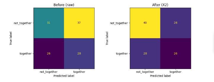
Graph showing before and after feature engineering

After feature engineering but now with pair features like height difference, MBTI distance, compatibility rank, hair/eye matches:

• ROC AUC jumps to 0.57

• Balanced accuracy goes to 0.53
  And the confusion matrix tells the story:

• Correct class not together predictions go from 31 to 40

• False positives drop from 37 to 28

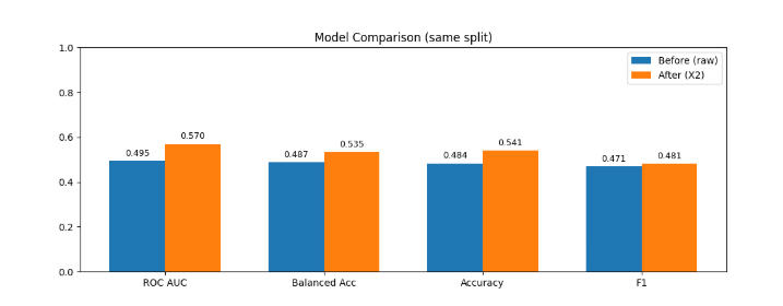
Now, someone will look at that and go: “0.49 to 0.57? That’s not huge.” Because those “small” improvements are literally real cases of changing sides.

It’s the difference between:

• flagging 9 fewer people incorrectly, and

• the model actually picking up patterns it was missing completely.

And if this was something high-stakes(like cancer screening) these aren’t just numbers on a chart.
A false positive means unnecessary panic, follow-up scans, biopsies, cost.
A false negative means you miss someone who actually needed treatment.

So yeah — the improvement looks “small” on paper, but in the real world, moving even a few cases in the right direction can be everything.

And the best part?
We didn’t change the model.
We didn’t get more data.
We didn’t use some fancy deep learning trick.

We just stopped feeding it trash inputs. 

THAT is the power of feature engineering.

For more of this, come on the journey with us and keep being Evil