
How does a computer see hair?
Have you ever wondered how computers can do this? Today we’re going to learn exactly how to do that.
Detecting someone’s hair colour from an image sounds simple.
Just find the colour of the hair and you’re done.
But when I tried to automate this, the results were completely wrong.
Sometimes the algorithm detected a yellow wall as blonde hair. Other times it picked up a brown shirt instead of the hair.
The problem wasn’t the colour detection.
The real problem was that the computer didn’t actually know where the hair was in the image. And solving that problem turns out to be much harder than it sounds.
You and I can instantly look at this image and understand where the hair is. Our brains separate the face, the background, the clothes, and the hair without thinking about it.
But how does a computer understand that?
From Pixels to Perception: How Computers Understand Images
How does it know which pixels belong to hair and which ones belong to a wall, a shirt, or the background?
And more importantly, how does it calculate that information?
We need to understand:
how computers represent images
how Convolutional Neural Networks detect visual patterns
and why segmentation models like BiSeNet are the key to solving this problem.
So let’s start from the beginning.
How does a computer actually see an image?
A computer represents an image as a grid of pixels. A pixel is the smallest unit of a digital image, representing a single point of colour in the image grid. More pixels usually means more detail and sharper quality, but it also increases the file size.

Evil Works Logo pixelated
Computers don’t “see” colours the way we do. They store each pixel as numbers (which are ultimately represented in binary). In the most common format, those numbers are in RGB, where every pixel is a mix of red, green, and blue intensities.
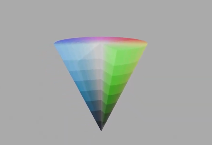
HSV Color Model
Finding Hair in Pixels: Colour, Context, and CNNs
For hair colour though, RGB isn’t always the easiest to work with, because lighting can change those values a lot. That’s why we switch to HSV: Hue represents the colour type (like an angle around a colour wheel), Saturation is how strong or washed-out that colour is, and Value is the brightness. For distinguishing hair shades like blonde, brown, and silver, HSV maps much more naturally to how humans describe colour.
But we’re getting ahead of ourselves.
Before we can talk about hair colour, we first need to answer a more basic question: how does the computer even know which pixels are hair?
That’s where Convolutional Neural Networks (CNNs) come in.
Convolutional Neural Networks were designed specifically for image processing. In many traditional machine learning approaches, images are first flattened into long vectors of numbers. When this happens, the model loses the spatial structure of the image and no longer knows which pixels were next to each other, making it harder to understand the image.
CNNs avoid this problem. Instead of flattening the image, they keep the pixel grid structure intact. This is important because in images the relationship between neighbouring pixels matters. Edges, shapes, and textures all depend on pixels being next to each other.
The core building block of a CNN is the convolutional layer.
Inside this layer, the network uses a small matrix called a filter (or kernel). This filter slides across the image from left to right and top to bottom. At every position, the filter is multiplied by the pixels underneath it. Mathematically, this operation is called convolution. For a small patch of the image, the output value is calculated as:
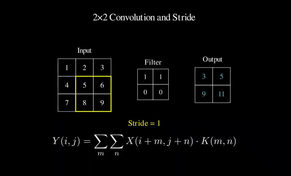
Convolutional Layer formula
Each filter in the network learns to detect a specific visual pattern. During training, the network adjusts the filter weights to capture useful signals in the data. Early layers usually learn simple features, such as:
edges
Lines
colour gradients
Deeper layers combine these simple patterns into more complex structures:
textures
Shapes
object parts
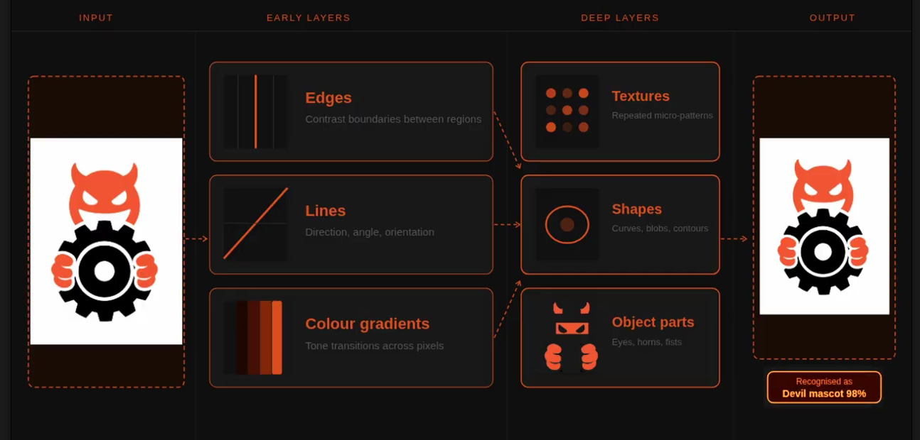
Features layers chart
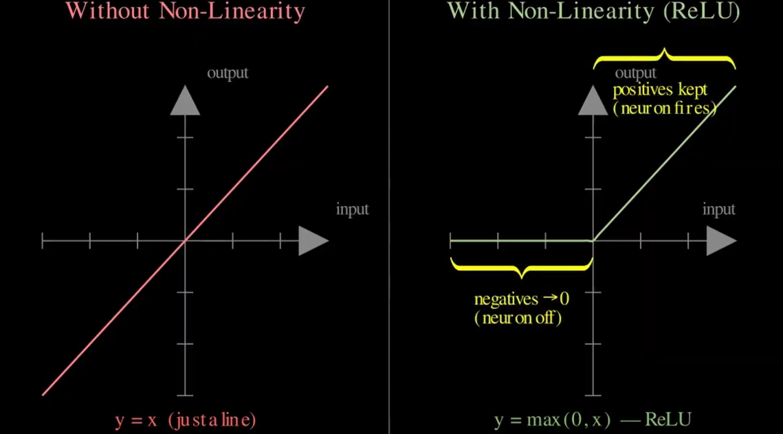
Eventually, the network can recognise entire objects. Mathematically, after convolution we apply a non-linear activation function, often ReLU:
This step introduces non-linearity, allowing the network to model complex patterns instead of just linear relationships.
The convolutional layer doesn’t use just one filter. It uses many filters simultaneously so it can learn from different features. If a layer has N filters, it produces N feature maps.
Non-linearity activation function
These maps are then stacked together to form a 3-dimensional tensor:
H×W×N
Where:
H= height
W = width
N = number of filters
Each slice of this tensor represents a different type of feature detected in the image. You can think of it as the network building a multi-perspective understanding of what’s inside the image.
But let’s stop and think about what we actually have here. Dozens of these feature maps, all stacked on top of each other. The network is rich with information perhaps too rich. So how do we take all of this and turn it into something the model can actually work with?
That's where pooling comes in.
Pooling reduces the spatial size of these feature maps, which helps:
reduce computation
reduce the number of parameters
focus on the most important signals
Instead of learning weights like a convolutional layer, pooling performs a fixed mathematical operation over small regions of the feature map. One common approach is average pooling. In average pooling, the network takes a small window of values and replaces it with their average.
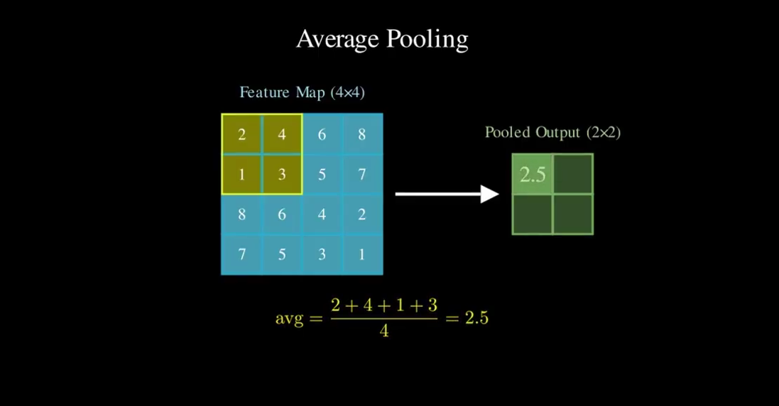
Average pooling function
Why We Need Segmentation…
Ok, Now that we understand how CNNs process images, let’s go back to our original problem.
For hair colour, the first question is: what part of the image are we measuring? There are three potential ways we can work this out.
Classification gives one label for the whole image (“blonde/brown/black”), but it can’t isolate hair. Background, clothes, and lighting can dominate the prediction.
Object detection draws a bounding box around a head/hair region, but the box still contains face, hat, sky, and background, so your “average colour” gets contaminated.
Segmentation labels pixels (or a mask) so you get only the hair pixels
That’s why segmentation is the better choice here: it lets you crop by mask instead of by box, so your colour calculation is based on the actual hair region, not everything near it.
Segmentation solves the problem conceptually: We label every pixel and isolate the hair region.
But this raises a new question:
How does a neural network actually learn which pixels belong to hair?
This is where modern segmentation architectures come in. One of the models designed specifically for this task is BiSeNet, short for Bilateral Segmentation Network.
BiSeNet was built to solve a key trade-off in image segmentation.
To correctly label pixels, a model needs two kinds of information at the same time:
Fine spatial detail — to detect precise edges and boundaries, like individual hair strands.
Global context — to understand what the object actually is, for example distinguishing hair from a brown wall or a shirt.
Most networks struggle because improving one often hurts the other.
If you downsample the image heavily, you gain context but lose detail.
If you keep high resolution, you preserve detail but the model struggles to understand the larger scene.
BiSeNet solves this by splitting the problem into two parallel paths.
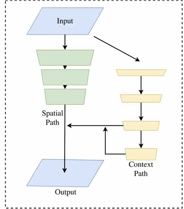
BiSeNet Architecture
BiSeNet Architecture - Spatial Path
The Spatial Path keeps the image resolution relatively high. Its goal is to preserve fine spatial information, such as:
hair edges
boundaries between hair and skin
small visual structures
It uses only a few convolution layers with stride 2, producing feature maps that are 1/8 the size of the original image.
Because the resolution stays relatively large, the network retains detailed spatial information.
Context Path
While the Spatial Path focuses on detail, the Context Path focuses on understanding the scene.
It uses a lightweight backbone network (like Xception) to quickly down sample the image and build a large receptive field.
A larger receptive field means the model can understand:
the head shape
where the face is
what parts belong to background vs person
To further capture global information, the network applies global average pooling, which summarizes the entire image.
This allows the model to understand the overall context of the scene.
Attention Refinement Module (ARM)
Inside the Context Path, BiSeNet introduces the Attention Refinement Module. This module uses global context to reweight important features. Mathematically, it:
Applies global average pooling
Produces an attention vector
Multiplies this vector with the feature map
The result is that the network focuses more on relevant semantic information.
Feature Fusion Module (FFM)
At this point the model has two very different types of information:
Spatial Path: detailed low-level features
Context Path: high-level semantic features
These cannot simply be added together.
So BiSeNet introduces a Feature Fusion Module, which learns how to combine them properly. The fused representation contains both:
precise boundaries
semantic understanding
From this combined representation, the network produces the final pixel-level prediction map. The output of the network is a segmentation map. It has the same width and height as the original image.
Each pixel receives a label:
parsing[y, x] = 17
Where the number corresponds to a class such as:
background
skin
eye
mouth
Hair
Once we know exactly which pixels belong to hair, the original problem becomes much easier.
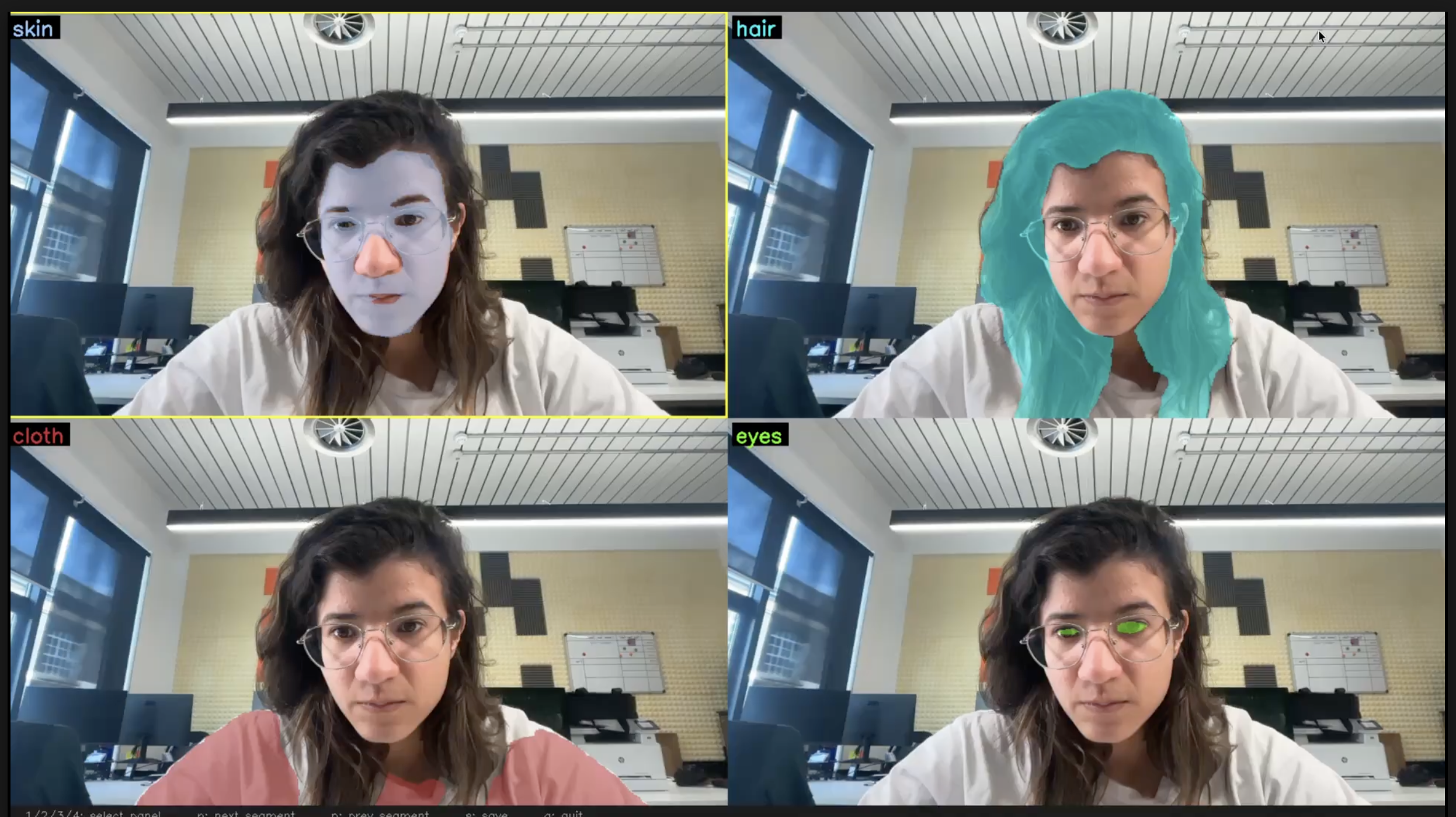
Computer vision with segmentation( top left: skin segment, top right: hair segment, bottom left: cloth segment and bottom right: eyes segment.
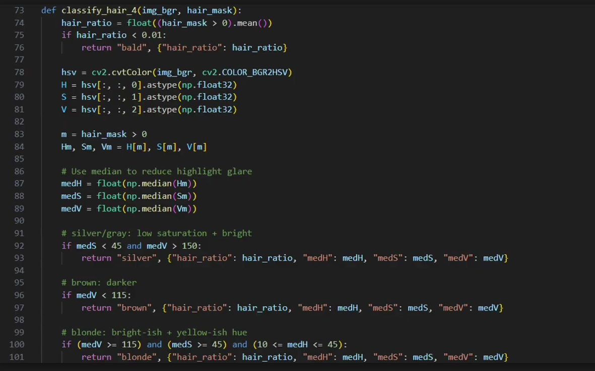
Function to classify the hair colour between: bald, silver', brown and blonde.
The Real Challenge Was Segmentation
Now we can simply:
Extract the pixels labelled as hair
Convert them to HSV
Compute the dominant colour
And that gives us a much more reliable estimate of a person’s hair colour. But the interesting part is that the hardest problem here wasn’t actually detecting colour.
It was teaching the computer where the hair is in the first place.
Once segmentation isolates the correct pixels, the colour calculation becomes almost trivial.
And this pattern appears everywhere in computer vision.
In self-driving cars, the system doesn’t just detect colours or shapes. It first has to segment the scene: road, pedestrians, traffic signs, vehicles.
In medical imaging, doctors don’t want an algorithm that simply says “tumour” or “no tumour.”
They need models that segment the exact region of the tumour so they can measure its size and growth.
The computer first needs to understand what part of the image belongs to what object. Only then can it measure, classify, or analyse it.
So in this project, detecting hair colour wasn’t really a colour problem. It was a segmentation problem. And once we solved that, the rest became simple math.
Because in machine learning, the hardest part is often not the prediction itself and it's teaching the model where to look.
For more of this, come on the journey with us and keep being Evil